You type the same command forty times a day and the tool just... knows. But knowing isn't the interesting part. The interesting part is how it forgets — with mathematical precision, at a rate you can calculate down to the decimal point. That's what Daniel's asking about this week. He sent in a whole thing about zoxide, the directory jumper we talked about recently, and he wants to go deeper on the concept that makes it work under the hood — decaying algorithms. Specifically, three questions. One, what actually is a decaying algorithm in plain terms? Two, how does zoxide's recency decay with that weighted bias actually function — what's the math doing? And three, where else does this same pattern show up in statistics and data visualization? He wants the concrete mechanism and then the zoomed-out view. So that's the arc — we start inside one Rust source file and end up in forecasting and heatmaps.

And I have to say, this is one of those topics where the implementation is genuinely elegant. I pulled the actual decay formula from zoxide's source code — it's in a file called util.rs — and it's one line. It's E raised to the power of negative elapsed hours times zero point five divided by eight thousand seven hundred sixty six. That's it. That single expression is the entire memory model.
Eight thousand seven hundred sixty six hours.
Which is exactly one year — three hundred sixty five point two five days. The zero point five in the numerator means the half-life is roughly one year. After twelve months without touching a directory, its score drops to about fifty percent of what it was.
So the tool has a sense of time that's literally baked into a constant. Somebody sat down and decided, a year feels right for how fast directory habits change.
And that decision is the whole ballgame. Change that constant and you change the personality of the tool. Make it a month and zoxide gets twitchy — it forgets everything you did before last Tuesday. Make it five years and it's basically a static bookmark system with extra steps.
Which is what most people's shell aliases already are.
The decay is what makes it adaptive rather than just... sedimentary. Layers of old paths piling up forever.
So let's start with the concrete. What is a decaying algorithm, stripped down?
Any function where the weight or influence of an observation decreases smoothly over time or distance. That's the definition. And the key word is smoothly — because there are other ways to make things forget. A sliding window, for example, just chops off everything older than some threshold. Day thirty one? Gone. Zero weight. Day thirty? Full weight, same as yesterday. That hard cutoff creates all kinds of weird edge-case behavior — a path you used constantly for months vanishes from consideration the instant it crosses the boundary.
Whereas decay never slams the door. It just... dims the lights.
Right. And the other alternative is uniform weighting — every observation counts equally forever. That's stable, but it can't adapt. If you change jobs and start working in a completely different directory tree, uniform weighting would keep suggesting your old paths for months because they have so much accumulated history.
So decay is the compromise. You get to adapt without catastrophically forgetting.
That's the tension. Stability versus responsiveness. Every system that learns from data has to pick a point on that spectrum, and decay is how you implement the middle ground with math rather than heuristics.
And Daniel's prompt is specifically about recency decay with a weighted bias. That phrase — weighted bias — what's it doing there?
It means the decay doesn't just happen passively. Every time you access a path, the clock resets on that entry — the score gets bumped up, and then decay starts eating away at it again from that new higher point. The bias is toward things you use frequently. A path you visit every day never gets a chance to decay meaningfully between accesses. A path you visited once six months ago has been decaying the whole time. The system isn't just tracking what you did — it's tracking the pattern of what you keep doing.
Use it or lose it, expressed as an exponential function.
And the "statistically predictable" part Daniel mentioned — that's crucial. This isn't a heuristic where someone said "eh, cut the score in half after a while." The decay follows a known mathematical function. You can calculate exactly what the score will be at any future point, given the access history. That predictability is what makes the behavior trustworthy. The tool won't surprise you with weird ranking choices — if something dropped off, you can compute why.
Alright, walk me through the actual formula. You said you pulled it from the source.
The expression is E to the power of negative elapsed hours times zero point five divided by eight seven six six. Let me break that down piece by piece. E is Euler's number — about two point seven one eight — and raising E to a negative power gives you exponential decay. The exponent has three components. Elapsed hours is time since the last access. The zero point five is ln of two — the natural log of two, which is about zero point six nine three — and dividing by the half-life in hours converts that to a decay constant.
Wait, say that part again. The zero point five is standing in for the natural log of two?
It's an approximation. The exact decay constant lambda would be ln of two divided by the half-life. Ln of two is roughly zero point six nine three. The zoxide author used zero point five instead, which gives a slightly slower decay than a true one-year half-life. It's close enough for a directory jumper — we're not launching satellites here.
So the half-life is actually a bit longer than a year, if the constant is smaller than the true ln of two.
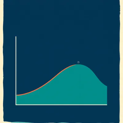
About fourteen months, if you work backward. But the principle is identical. The important thing is the shape of the curve, not the exact constant. And the shape is exponential decay — steep at first, then a long gradual tail.
Which means a path loses a lot of its score in the first few months, and then the decline slows down.
Yes. After one half-life, fifty percent remains. After two half-lives, twenty-five percent. After three, twelve and a half. It never quite reaches zero, mathematically — but practically, after five or six half-lives, the score is negligible.
And the "weighted bias" part — that's the access bump?
Right. Every time you visit a path, zoxide adds to its score. The exact increment depends on the ranking algorithm — zoxide has a few modes — but the core idea is that each access adds a fixed amount, and then decay multiplies the accumulated score by that exponential factor continuously. So the score at any moment is the sum of past accesses, each discounted by how long ago it happened.
So if I visit slash home slash projects every day, each of those daily visits is contributing, but yesterday's visit counts for nearly full weight while the visit from three months ago is heavily discounted.
And the visits from six months ago are barely a whisper. But they're not zero. That's the difference from a sliding window — the old data never fully disappears, it just becomes increasingly irrelevant. In a sliding window, the visit from day thirty one is exactly as gone as the visit from day three hundred.
Let's make this concrete. Give me a simulation.
Alright. Imagine two paths. Path A — you access it every day for the first seven days, then never again. Path B — you access it once, on day twenty nine. We're tracking thirty days total. For simplicity, let's say each access adds one point, and we'll use a half-life of... let's say ten days to make the numbers move faster.
Ten days, so the decay constant is ln of two over ten, about zero point zero six nine per day.
Day one, path A gets accessed, score goes to one. Day two, that one has decayed to about zero point nine three, then you access again, score goes to one point nine three. Day three, the accumulated score decays to about one point eight, plus another access, now two point eight. By day seven, after seven daily accesses, the score is roughly... let me think... each day you're adding one and the previous days are decaying. The score converges toward a steady state where the decay between visits exactly balances the one-point increment. With daily access and a ten-day half-life, the steady state is around fourteen or fifteen points.
Because the decay per day is only about seven percent, so you need a lot of accumulated score before the daily loss equals one point.
So after day seven, path A has roughly fifteen points and then... abandonment. No more accesses. Day eight, it decays by seven percent — down to about fourteen. Day fifteen, it's down to about nine. Day twenty nine, it's down to about three point two.
Meanwhile path B gets its one access on day twenty nine and scores one point.
Right. So even after three weeks of abandonment, the path you used heavily for one week still outranks the path you touched once yesterday. That's the weighted bias at work — frequency matters, not just recency. The score encodes both.
Which feels right, intuitively. A directory you lived in for a week is probably more relevant than one you poked at once, even if the poke was more recent.
And that's the design choice. If zoxide only cared about recency, it would just sort by last access time and be done. The decay-weighted accumulation is what gives it a memory that's more nuanced than "what did you do most recently."
Now, you said this is the same math as radioactive decay.
Identical. Carbon-fourteen dating uses exactly the same formula — N of t equals N zero times E to the negative lambda t. Carbon-fourteen's half-life is five thousand seven hundred thirty years. Zoxide's effective half-life is about a year. The math doesn't care about the timescale. It's the same differential equation — the rate of change is proportional to the current amount.
And capacitor discharge.
Also exponential. An RC circuit discharges with time constant tau equals R times C. After one time constant, the voltage is down to about thirty-seven percent of the original — that's one over E. After five time constants, it's below one percent. Same curve, different physical system.
Drug metabolism too, right? This is where your clinical background...
Pharmacokinetics, yes. Many drugs are eliminated from the bloodstream following first-order kinetics — exponential decay. The half-life of caffeine is about five hours in most adults. Ibuprofen, about two hours. The dosing schedule is designed around that decay — you take the next dose before the concentration drops below the therapeutic threshold. It's literally the same math as zoxide deciding when a directory falls below the relevance threshold.
So an anesthesiologist calculating a propofol drip and a Rust CLI tool deciding which directory to jump to are solving the same equation.
They're tuning the same parameter — half-life — to match the natural timescale of the system they're working with. For propofol, the half-life is minutes. For directory habits, it's months. The equation doesn't change.
Alright, let's zoom out. Daniel's third question was about where else this pattern appears in statistics and data visualization. You mentioned exponential smoothing.
This is where it gets really good. Exponential smoothing is a family of forecasting methods, and the most famous variant is Holt-Winters. It decomposes a time series into three components — level, trend, and seasonality — and applies a separate decay parameter to each one.
Three different half-lives, essentially.
Three different smoothing parameters, conventionally called alpha, beta, and gamma. Each is between zero and one. Alpha controls how fast the estimated level adapts to new observations. Beta controls how fast the trend adapts. Gamma controls how fast the seasonal pattern adapts. And they all work the same way — each new observation updates the estimate by blending the old estimate with the new data point, weighted by the parameter.
So if alpha is zero point three, the new level estimate is thirty percent the new observation and seventy percent the old estimate.
And here's where the decay becomes visible. That blending means the weight of an observation from k periods ago is alpha times one minus alpha to the power of k. It's exponential decay in the weight assigned to historical data. If alpha is zero point three, an observation from one period ago has weight zero point three. Two periods ago, zero point three times zero point seven, which is zero point two one. Three periods, zero point one four seven. Six periods, it's down to about twelve percent of the original weight.
So the half-life in terms of periods is ln of two divided by negative ln of one minus alpha. For alpha equals zero point three, that's about... two periods?
About two point four periods. After two or three observations, the influence of old data is already cut in half. And that's the tuning decision — if your time series changes rapidly, you want a high alpha so the model forgets quickly. If it's stable, low alpha, long memory.
This is exactly the same tradeoff as zoxide's half-life constant. Fast adaptation versus stability.
It's the same tradeoff in every domain. Bayesian statistics has a version of this called exponential forgetting. When you're tracking a distribution that changes over time — stock market volatility, user preferences, network traffic patterns — you can't just accumulate all historical data equally. You apply a decay factor to the prior, so old observations contribute exponentially less to the posterior. After N half-lives, the data is effectively gone from the model's working memory.
Concept drift. The thing your spam filter deals with when spammers change tactics.
A spam filter trained on emails from twenty eighteen would be terrible today if it weighted everything equally. But with exponential forgetting, it continuously adapts — old patterns fade, new patterns dominate. The half-life parameter determines how quickly it pivots.
And if you set it wrong, you get either a filter that's stuck in twenty eighteen or one that panics every time it sees a slightly unusual email.
The Goldilocks problem. Too fast, and the model chases noise — it overreacts to every outlier. Too slow, and it misses real shifts. There's no universal right answer — the half-life has to match the phenomenon.
Which brings us to data visualization. Daniel asked specifically about that.
Kernel density estimation is the cleanest example. KDE takes a scatter of discrete points and produces a smooth continuous density surface — it answers the question "where are points most concentrated?" And it does it by placing a kernel function at each data point and summing them up.
A kernel being a little bump of influence.
A probability distribution, typically a Gaussian. The Gaussian kernel assigns weight to nearby points according to E to the negative x squared over two h squared, where h is the bandwidth parameter. That's the decay rate. Points close to the center get near-full weight. As distance increases, weight drops off following a Gaussian curve — which is exponential decay with a squared term in the exponent.
So h is the spatial half-life, essentially.
It's the standard deviation of the kernel. A small h means the kernel is narrow — influence decays rapidly with distance. You get a spiky, detailed density estimate that picks up every local cluster. A large h means the kernel is wide — influence decays slowly. You get a smooth, broad density estimate that shows only the largest-scale patterns.
Overfitting versus oversmoothing.
Same tradeoff again. And you can see it immediately when you plot the same data with different bandwidths. With h equals zero point five, you might see five distinct peaks corresponding to five clusters in the data. With h equals two point zero, those five peaks merge into one or two broad humps. The decay rate literally controls what story the visualization tells.
So choosing a bandwidth is an editorial decision, whether the analyst admits it or not.
The default bandwidth selection methods — Scott's rule, Silverman's rule — they're attempts to automate that editorial decision based on the data's variance and sample size. But the defaults make assumptions about the underlying distribution that may not hold. A responsible visualization always includes a sensitivity check — what does this look like at half the bandwidth? Double?
Heatmaps do something similar, right?
Same principle. Tools like matplotlib's hexbin or seaborn's kdeplot are creating density estimates from discrete points. The "smoothness" parameter in those functions is literally a decay rate. Too fast a decay and you get a heatmap that's mostly empty space with a few hot pixels. Too slow and everything blurs into a uniform glow.
The hexbin one is interesting because it's discretizing space into hexagons first, and then applying what's essentially a spatial decay to smooth across bins.
The bin size interacts with the smoothing bandwidth. Large bins with wide smoothing — you lose all local structure. Small bins with narrow smoothing — you get noise amplified into features. The art is balancing the two so the visualization reveals genuine patterns at the scale that matters for the question you're asking.
I want to pull on a thread here. In zoxide, decay is temporal — it's about time since last access. In KDE, decay is spatial — distance in feature space. In exponential smoothing, decay is sequential — position in the time series. Three different independent variables, same exponential family.
That's the insight. The math is identical. The only thing that changes is what you're measuring distance from. In zoxide, distance is hours elapsed. In KDE, distance is Euclidean space. In Holt-Winters, distance is lag — how many periods back in the sequence. But the function that maps distance to weight is the same shape every time.
Which means if you understand one of these systems, you have intuition for all of them. The tuning parameter might be called half-life, or bandwidth, or alpha, or smoothing factor — but it's always answering the same question. How fast should influence decay with distance?
And "distance" itself is a design choice. You could imagine a zoxide variant where decay is spatial — directories that are nearby in the filesystem tree get higher weight. Or a version where decay is based on how many other directories you've visited in between — sequential distance rather than temporal. Each choice encodes a different theory of what makes a directory relevant.
The current zoxide assumes temporal distance is the right metric. Recent is relevant.
Which is usually true but not always. If you're working on a quarterly report, the relevant directories might be the ones you used three months ago, not the ones you used yesterday. The decay model has no way to know about that cyclic pattern.
Unless you add seasonality — which is exactly what Holt-Winters does. The gamma parameter captures periodic patterns on top of the level and trend.
Right. And you could imagine a zoxide that learns your weekly or monthly cycles. Monday mornings you always hit the sprint planning directory. End of month you always hit the invoicing directory. A pure temporal decay model misses that. But a seasonal decay model would boost those paths right before their predicted access time.
Has anyone built that?
Not that I've seen in a directory jumper. But the math exists. It's just Holt-Winters applied to filesystem paths instead of sales figures.
Alright, let's land some of this. What do we actually do with this knowledge?
Three things. First, when you're designing any adaptive system — recommendation engines, anomaly detection, cache eviction — prefer exponential decay over sliding windows. Sliding windows create hard boundaries where behavior changes discontinuously. Day thirty one is treated as fundamentally different from day thirty, even if nothing meaningful changed. Decay is smooth — there's no cliff edge for edge-case bugs to hide behind.
I've seen cache eviction policies that use exact TTLs and the moment something expires, the cache hit rate falls off a cliff for that item. A decay-based eviction would just gradually demote it.
You avoid the thundering herd problem where everything expires simultaneously and suddenly your database gets hammered. Decay staggers the effective expiration naturally.
Second takeaway?
The half-life parameter is your most important tuning knob, and you need to match it to the natural timescale of what you're modeling. Zoxide chose roughly a year because directory habits change on the order of months. A news recommendation system might use hours — if you're not showing me stories about something that happened this morning, you're stale. An earthquake detection system might use seconds. The question is always: how fast does the underlying reality change? Set your half-life to match.
If you don't know, err on the side of longer. A system that adapts too slowly is just sluggish — it still works, it's just behind. A system that adapts too fast is chaotic — it chases noise and the user loses trust.
That's the clinical parallel again. You titrate the dose. Start conservative, observe the response, adjust.
Third takeaway?
Audit the decay assumptions in tools you already use. Your email spam filter has a decay rate. Your music recommendation algorithm has a decay rate. Your shell history — if you use something like Atuin or the default bash history with HISTSIZE — it's using a form of decay, even if it's just truncation. Understanding the math lets you predict when these systems will fail. If your behavior changes faster than the decay rate can adapt, the system will serve you stale recommendations until enough new data accumulates to overcome the old weights.
The moment you switch from listening to metal to listening to jazz, your recommendation algorithm is fighting its own decay function. It's still weighted toward the old genre until the new listens accumulate enough mass.
You can calculate roughly how long that'll take. If the half-life is thirty days and you listened to metal for two years, you've got a lot of accumulated weight to overcome. The algorithm isn't broken — it's working exactly as designed. The design just doesn't match your new reality yet.
The frustration people feel with recommendation systems is often just the half-life parameter being wrong for their rate of change.
Or the system not having a mechanism to detect phase shifts — sudden genuine changes in preference versus gradual drift. Some systems add a change-detection layer that temporarily shortens the half-life when prediction error spikes. That's getting into more sophisticated territory, but the principle is still decay — just with an adaptive rate.
Before we close out, I want to poke at one assumption. Everything we've talked about is exponential decay. But there are other decay functions. Power-law decay, for example — where weight drops off as one over t to some power instead of E to the negative lambda t. Or logistic decay, which is S-shaped. Why don't we see those in tools like zoxide?
Exponential decay has a special property that makes it mathematically convenient — it's memoryless. The conditional probability of decay in the next interval doesn't depend on how long you've already waited. For a directory jumper, that means the decay rate is constant regardless of the path's age. A path that's six months old decays at the same percentage rate as a path that's two years old.
Whereas power-law decay would mean old paths decay more slowly — they have a longer tail.
Right. Power-law decay is actually closer to how human memory works — we forget rapidly at first, then what survives tends to stick around for a long time. The forgetting curve Ebbinghaus documented in the eighteen eighties is roughly power-law. So there's a real argument that a directory jumper should use power-law decay, not exponential, if the goal is to model human memory patterns.
Or logistic decay, where there's a plateau at the beginning — you don't forget anything for a while — then a rapid drop, then another plateau of things you'll never forget.
Which maps to the difference between your working memory, your short-term memory, and your long-term memory. Different decay regimes for different memory systems.
The open question is: zoxide uses exponential decay because it's simple and mathematically clean. But what would a directory jumper look like if it used a decay function that actually matched human forgetting? Would it feel more natural? Or would the mathematical convenience of exponential decay win out because predictability matters more than biological fidelity?
That's a interesting design question. And it connects to something bigger. As AI tools start incorporating more sophisticated memory mechanisms — attention decay in transformers, forgetting in continual learning systems, episodic memory in agents — the choice of decay function becomes a design decision with real consequences. Understanding the difference between exponential, power-law, and logistic decay isn't just academic. It's how you debug why an AI system remembers some things and forgets others.
The same way you debug why zoxide keeps suggesting a directory you haven't used in eight months.
Check the half-life. Check the access history. The math tells the story.
This has been My Weird Prompts. Thanks to our producer Hilbert Flumingtop for making this whole thing run.
If this episode made you think differently about how your tools forget — or remember — send us your weird prompt. The address is show at my weird prompts dot com. We read everything.
We'll be back soon.